Monday, March 14/Tuesday, March 15
Submissions due to turnitin.com by Monday, March 21 @11:59 p.m.
Submissions due to turnitin.com by Monday, March 21 @11:59 p.m.
Submissions due to turnitin.com by Monday, March 21 @11:59 p.m.
Submissions due to turnitin.com by Monday, March 21 @11:59 p.m.
Submissions due to turnitin.com by Monday, March 21 @11:59 p.m.
Submissions due to turnitin.com by Monday, March 21 @11:59 p.m.
Submissions due to turnitin.com by Monday, March 21 @11:59 p.m.
Submissions due to turnitin.com by Monday, March 21 @11:59 p.m.
Submissions due to turnitin.com by Monday, March 21 @11:59 p.m.
Submissions due to turnitin.com by Monday, March 21 @11:59 p.m.
Submissions due to turnitin.com by Monday, March 21 @11:59 p.m.
Submissions due to turnitin.com by Monday, March 21 @11:59 p.m.
Submissions due to turnitin.com by Monday, March 21 @11:59 p.m.
Submissions due to turnitin.com by Monday, March 21 @11:59 p.m.

Submissions due to turnitin.com by

Check the exemplar to make sure you have the right calculations, formatting, etc. before submitting.
INCORRECT CALCULATIONS WILL RESULT IN AN AUTOMATIC 50% OR LOWER.
ALL ASSIGNMENTS WILL BE CHECKED FOR INTEGRETIY. STUDENTS WHO SUBMIT WORK THAT IS NOT THEIR OWN WILL RECIEVE A ZERO AS WILL THE SHARING STUDENT.
Learning Targets:
Students will be able to:
- create a spreadsheet that calculates commission, bonus pay, net pay, and statistical information.
- check their work for calculation errors and make corrections if necessary.
Resources:
- Lesson: Myers Staffing: Employees on Commission
- You will use this image to SET UP your spreadsheet:
![]()
NOTE:
- Font: Calibri
- Row 2: size 20
- Row 3: size 18
- Rest: size 12
- Row 2 click the merge and center button to combine the cells in the row.
- Do the same for row 3.
- For the titles in row 5, apply WRAP TEXT to get the text on two lines–this is dependent on how wide your column is.
- Enter the text and data as shown in the example below.
- Add similar borders and shading as shown in the example below.
- You may select your own colors, but they must be consistent with the example and I must be able to see your text.
- Formulas are discussed in the lesson video posted above–You must watch it to find out what they are!
- Add your first and last name in cell B29.
CHECK YOUR WORK:
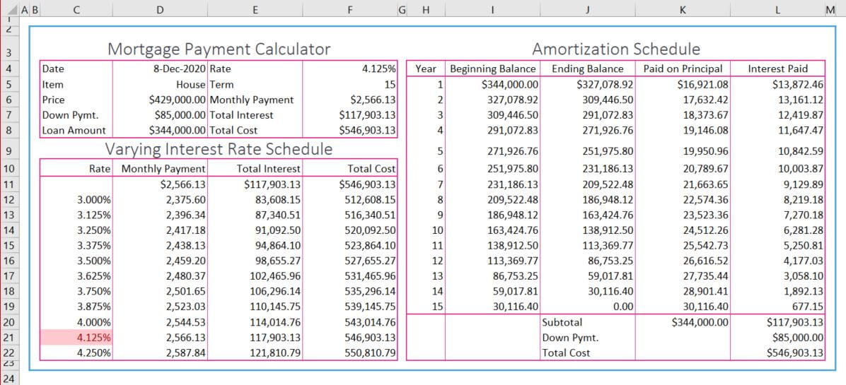
Click the image below to view the finished product:

Myers Staffing, INC.: Employees on Commission
- Attendance.
- Independently view the lesson in the Resource section above BEFORE beginning the spreadsheet.
- Independently create the Myers Staffing Inc., Employees on Commission spreadsheet in the DESKTOP version of Excel. This means from your own computer OR the remote server.
- Save often and save before you submit.
- When you have finished, you will check your document over for correct formatting, spelling, etc.–INCORRECT CALCULATIONS WILL RESULT IN A 50% OR LOWER GRADE. TYPING NUMBERS INSTEAD OF FORMULAS WILL EARN YOU A ZERO. ALL ASSIGNMENTS WILL BE CHECKED FOR INTEGRETIY. STUDENTS WHO SUBMIT WORK THAT IS NOT THEIR OWN WILL RECIEVE A ZERO AS WILL THE SHARING STUDENT.
- You will then submit to turnitin.com. Submissions due to turnitin.com by Monday, March 1 by 3:40 p.m.
Performance of Understanding:
- Myers Staffing, Inc.: Employees on Commission (LastNameCommission)